FGPG_V11 ::: Introduce of Fine Involute Gear Tooth Profile Generator

FGPG_V11


새로운 인볼류트 기어 설계용 프로그램을 작성해 보았다.
기존의 GPG_V08을 대체한다는 의미로 FGPG 라고 이름을 붙였다.
Fine Gear Profile Generator 의 줄임말이다.
아직 미완성본이지만, 일단 필요한 기능들은 대부분 어설프게나마 다 구현되었으므로 기록 차원에서 올려본다.

특징은 대략 다음과 같다.

1. Julia Language로 작성되었다.
2. 아직 독립 실행파일(Standalone Executable)은 빌드하지 않았다.
3. Julia를 이용하여 Python MatPlotLib의 플랏팅 능력을 활용한다.
4. Gmsh 및 Elmer를 이용하여 자동적으로 FEM 해석을 실시해 주는 Batch 파일을 만들어준다.  윈도우용 뿐만 아니라, 리눅스용 Shell Script도 만들어지므로 운영체제에 상관없이 사용 가능하다.
5. 입력하는 파라미터들은 별도의 파일로 작성해 두면, 그것을 읽어서 계산해 낸다.
6. GUI는 없다.
7. AutoCAD 또는 DraftSight에서 기어 형상을 자동으로 그려줄 수 있도록 Script 파일이 자동으로 생성된다.  여기서 dxf 파일로 저장한 후, 3D CAD 에서 모델링 할 수 있다.


우선 프로그램의 소스코드는 다음과 같다.
파일 이름은 FGPG_V11.jl 이다.  다른 이름을 붙여도 상관없다.

#########################################################################
# FGPG (Fine_Gear_Profile_Generator) V11
# 20150602
# by Dongho Kim  from Korea
# dymaxion.kim@gmail.com
# http://dymaxionkim.blogspot.kr/
#########################################################################
## Ref.
# http://tro.kr/29
# http://en.wikipedia.org/wiki/Coordinate_rotations_and_reflections
# http://dip28p.web.fc2.com/
#########################################################################
## History
# 20141114 V0.44 : SageMath Version
# 20150519 V0.1 : Trying to Conversion for Julia, Trying Interact Macro
# 20150519 V0.2 : Studying about Lack
# 20150527 V01 : Plotting Whole Gear at first
# 20150527 V02 : Trying Interact Macro
# 20150527 V03 : Debug V01
# 20150527 V04 : Adding Annotations, Saving Profile Data File, ...
# 20150527 V05 : Adding More Error Checks, Making geo File
# 20150528 V06 : Debug Making geo File
# 20150528 V07 : Align vertically Gear, Add Shaft
# 20150528 V08 : Modifying Sequences, Debug Making geo File, Make new Figure, Make svg Pictures, Save scr File, Modify Annotations
# 20150530 V09 : Modifying Shaft, Internal-External Condition, geo File
# 20150531 V10 : Adding version Variable
# 20150602 V11 : Making case.sif, case.bat, case.sh files
#########################################################################
## Todo
# Write Theory Doc
# Write User Manual
# Write Some Actual Examples
# Tip Relief to Modifying Tooth Profile
# Making Spec Table
# Making case.sif
# Profile Repairing in Undercut Condition
# Technical Error Check & Anouncing
# Change Variable Names for easy code reading
# Re-code in Functional Criteria (?)
# Wndows Batch File
# Bash Script
# Change Result File Name based in Time
# Build to Standalone Executable

# On JUNO envirenment
cd(dirname(@__FILE__))

using PyPlot
PyPlot.svg(true)

############################
# Parameters
version = "v11"
m = 1  # Module
z = 20  # Teeth Number
alpha_0_deg = 20  # Pressure Angle [Deg]
x = 0.2  # Offset Factor
b = 0  # Backlash Factor
a = 1.0  # Addendum of Tooth
d = 1.2  # Dedendum of Tooth
c = 0.3  # Radius Factor of Edge Round of Hob
e = 0.2  # Radius Factor of Edge Round of Tooth
# Center of Gear
x_0 = 0
y_0 = 0
# Segmentation Points Numbers for each curves
seg_circle = 360
seg_involute = 50
seg_edge_r = 4
seg_root_r = 20
seg_center = 2
seg_outter = 4
seg_root = 4


############################
# Input Parameters from input4fgpg.csv file
input4fgpg = readcsv("input4fgpg.csv")
input4fgpg[:,3] = float64(input4fgpg[:,3])
m = input4fgpg[1,3]
z = int64(input4fgpg[2,3])
alpha_0_deg = input4fgpg[3,3]
alpha_0 = alpha_0_deg*2*pi/360
x = input4fgpg[4,3]
b = input4fgpg[5,3]
a = input4fgpg[6,3]
d = input4fgpg[7,3]
c = input4fgpg[8,3]
e = input4fgpg[9,3]
x_0 = input4fgpg[10,3]
y_0 = input4fgpg[11,3]
seg_circle = int64(input4fgpg[12,3])
seg_involute = int64(input4fgpg[13,3])
seg_edge_r = int64(input4fgpg[14,3])
seg_root_r = int64(input4fgpg[15,3])
seg_center = int64(input4fgpg[16,3])
seg_outter = int64(input4fgpg[17,3])
seg_root = int64(input4fgpg[18,3])


############################
# Involute Curve
# alpha_m = Center Line's Slope [Rad]
alpha_m = pi/z
# alpha_is = Start Angle for Involute Curve
alpha_is = alpha_0 + pi/(2*z) + b/(z*cos(alpha_0)) - (1+2*x/z)*sin(alpha_0)/cos(alpha_0)
# theta_is = Minimum Range of Parameter to Draw Involute Curve
theta_is = sin(alpha_0)/cos(alpha_0) + 2*(c*(1-sin(alpha_0))+x-d)/(z*cos(alpha_0)*sin(alpha_0))
# theta_ie = Maximum Range of Parameter to Draw Involute Curve
theta_ie = 2*e/(z*cos(alpha_0)) + sqrt( ((z+2*(x+a-e))/(z*cos(alpha_0)))^2 - 1 )
# Condition of theta_ie
if alpha_malpha_m && alpha_m>alpha_is+theta_ie-atan(theta_ie)
    e = (z/2)*cos(alpha_0)*( theta_ie - sqrt( (1/cos(alpha_is+theta_ie-alpha_m))^2-1 ) )
end
# x_e, y_e = Location of Tooth's End Point
x_e = x_0 + m*((z/2)+x+a)*cos(alpha_e)
y_e = y_0 + m*((z/2)+x+a)*sin(alpha_e)
# x_e0, y_e0 = Location of Edge Round Center
x_e0 = m*(z/2+x+a-e)*cos(alpha_e) + x_0
y_e0 = m*(z/2+x+a-e)*sin(alpha_e) + y_0
# Parameter Range of Edge Round
theta3_min = atan((Y1[length(Y1)]-y_e0)/(X1[length(X1)]-x_e0))
theta3_max = atan((y_e-y_e0)/(x_e-x_e0))
THETA3 = linspace(theta3_min,theta3_max,seg_edge_r)
X3 = m*e*cos(THETA3)+x_e0
Y3 = m*e*sin(THETA3)+y_e0
#plot(X3,Y3,color="green",linestyle="-")


############################
# Root Round Curve of Tooth
# Condition Check
# alpha_ts = Start Angle of Root Round Curve
# THETA_s = Substitution Variable to plot Root Round Curve
alpha_ts = (2*(c*(1-sin(alpha_0))-d)*sin(alpha_0)+b)/(z*cos(alpha_0)) - 2*c*cos(alpha_0)/z + pi/(2*z)
theta_te = 2*c*cos(alpha_0)/z - 2*(d-x-c*(1-sin(alpha_0)))*cos(alpha_0)/(z*sin(alpha_0))
THETA_t = linspace(0,theta_te,seg_root_r)
if c!=0 && (d-x-c)==0
    # mc를 반지름으로 하는 원호를 그려서 대체하게 됨
    THETA_s = (pi/2)*ones(length(THETA_t))
    elseif c==0 && (d-x-c)==0
    # 루트커브 작도 생략하고, (x_is,y_is) 점을 대칭으로 이뿌리호를 그려서 대체하게 됨
    elseif (d-x-c)!=0
    THETA_s = atan((m*z*THETA_t/2)/(m*d-m*x-m*c))
end
X_t = x_0 + m*( (z/2+x-d+c)*cos(THETA_t+alpha_ts) + (z/2)*THETA_t.*sin(THETA_t+alpha_ts) - c*cos(THETA_s+THETA_t+alpha_ts) )
Y_t = y_0 + m*( (z/2+x-d+c)*sin(THETA_t+alpha_ts) - (z/2)*THETA_t.*cos(THETA_t+alpha_ts) - c*sin(THETA_s+THETA_t+alpha_ts) )
#plot(X_t,Y_t,color="green",linestyle="-")


############################
# Outter Arc
#alpha_em = 2*alpha_m-alpha_e
#x_em = x_0 + m*(z/2+x+a)*cos(alpha_em)
#y_em = y_0 + m*(z/2+x+a)*cos(alpha_em)
THETA6 = linspace(alpha_e,alpha_m,seg_outter)
X6 = m*(z/2+a+x)*cos(THETA6)+x_0
Y6 = m*(z/2+a+x)*sin(THETA6)+y_0
#plot(X6,Y6,color="red",linestyle="-")


############################
# Root Arc
#x_rm = x_0 + m*(z/2+x-d)*cos(alpha_ts)
#y_rm = y_0 - m*(z/2+x-d)*sin(alpha_ts)
THETA7 = linspace(0,alpha_ts,seg_root)
X7 = m*(z/2-d+x)*cos(THETA7)+x_0
Y7 = m*(z/2-d+x)*sin(THETA7)+y_0
#plot(X7,Y7,color="red",linestyle="-")


############################
# Combine Curves
# Not using Root Round Curve (X_t,Y_t)
if c==0 && (d-x-c)==0
    Xc = X7[1:length(X7)-1]
    Yc = Y7[1:length(Y7)-1]
else
    Xc = [ X7[1:length(X7)-1]; X_t[1:length(X_t)-1] ]
    Yc = [ Y7[1:length(Y7)-1]; Y_t[1:length(Y_t)-1] ]
end
# Not using Edge Round Curve (X3,Y3)
if e==0 || alpha_m==alpha_is+theta_ie-atan(theta_ie)
    Xc = [ Xc; X1[1:length(X1)-1] ]
    Yc = [ Yc; Y1[1:length(Y1)-1] ]
else
    Xc = [ Xc; X1[1:length(X1)-1]; X3[1:length(X3)-1] ]
    Yc = [ Yc; Y1[1:length(Y1)-1]; Y3[1:length(Y3)-1] ]
end
# Not using Outter Arc (X6,Y6)
if alpha_e == alpha_m || alpha_m==alpha_is+theta_ie-atan(theta_ie)
    Xc = Xc
    Yc = Yc
else
    Xc = [ Xc; X6[1:length(X6)-1] ]
    Yc = [ Yc; Y6[1:length(Y6)-1] ]
end
#Xc = [ X7[1:length(X7)-1]; X_t[1:length(X_t)-1]; X1[1:length(X1)-1]; X3[1:length(X3)-1]; X6[1:length(X6)-1]]
#Yc = [ Y7[1:length(Y7)-1]; Y_t[1:length(Y_t)-1]; Y1[1:length(Y1)-1]; Y3[1:length(Y3)-1]; Y6[1:length(Y6)-1]]
#plot(Xc,Yc,color="black",linestyle="-",linewidth=2)



############################
# Make Whole One Tooth
Xc2 = Xc[2:length(Xc)]
Yc2 = Yc[2:length(Yc)]
# Reflect Transform
Xcc = cos(2*alpha_m)*(Xc2-x_0) + sin(2*alpha_m)*(Yc2-y_0)
Ycc = sin(2*alpha_m)*(Xc2-x_0) - cos(2*alpha_m)*(Yc2-y_0)
# Location Transform to (x_0,y_0)
Xcc = Xcc + x_0
Ycc = Ycc + y_0
# Invert
Xcc = Xcc[length(Xcc):-1:1]
Ycc = Ycc[length(Ycc):-1:1]
# Combine
Xcc = [Xc; Xcc]
Ycc = [Yc; Ycc]
#plot(Xcc,Ycc,color="black",linestyle="-",linewidth=2)


############################
# Align to Top
align_angle = pi/2-pi/z
X_align = Xcc
Y_align = Ycc
# Rotate
X_align = cos(align_angle)*(Xcc-x_0) - sin(align_angle)*(Ycc-y_0)
Y_align = sin(align_angle)*(Xcc-x_0) + cos(align_angle)*(Ycc-y_0)
# Location Transform to (x_0,y_0)
X_align = X_align + x_0
Y_align = Y_align + y_0
#plot(X_align,Y_align,color="black",linestyle="-",linewidth=2)


############################
# Make Whole Gear
p_angle = 2*pi/z
Xccc = X_align
Yccc = Y_align
Xtemp = X_align[2:length(X_align)]
Ytemp = Y_align[2:length(Y_align)]
for i = 1:z-1
    # Rotate
    Xtemp = cos(p_angle*i)*(X_align[2:length(X_align)]-x_0) - sin(p_angle*i)*(Y_align[2:length(Y_align)]-y_0)
    Ytemp = sin(p_angle*i)*(X_align[2:length(X_align)]-x_0) + cos(p_angle*i)*(Y_align[2:length(Y_align)]-y_0)
    # Location Transform to (x_0,y_0)
    Xtemp = Xtemp + x_0
    Ytemp = Ytemp + y_0
    Xccc = [Xccc; Xtemp]
    Yccc = [Yccc; Ytemp]
end



############################
# Plot Figure
f=figure(figsize=(10,10))
grid("on")
title("FGPG (Fine_Gear_Profile_Generator) $version \n by Dymaxion.Kim")
axis("equal")


############################
# Base, Pitch, Offset, Outter, Root Circle
THETA0 = linspace(0.0,2*pi,seg_circle)
# Base Circle
base_dia = m*z*cos(alpha_0)
X_base = base_dia/2*sin(THETA0) + x_0
Y_base = base_dia/2*cos(THETA0) + y_0
plot(X_base, Y_base, color="cyan", linestyle="--")
# Pitch Circle
pitch_dia = m*z
X_pitch = pitch_dia/2*sin(THETA0) + x_0
Y_pitch = pitch_dia/2*cos(THETA0) + y_0
plot(X_pitch, Y_pitch, color="magenta", linestyle="--")
# Offset Circle
offset_dia = 2*m*(z/2+x)
X_offset = (offset_dia/2)*sin(THETA0) + x_0
Y_offset = (offset_dia/2)*cos(THETA0) + y_0
plot(X_offset, Y_offset, color="red", linestyle="--")
# Outter Circle
outter_dia = 2*m*(z/2+x+a)
X_out = (outter_dia/2)*sin(THETA0) + x_0
Y_out = (outter_dia/2)*cos(THETA0) + y_0
plot(X_out, Y_out, color="brown", linestyle="--")
# Root Circle
root_dia = 2*m*(z/2+x-d)
X_root = (root_dia/2)*sin(THETA0) + x_0
Y_root = (root_dia/2)*cos(THETA0) + y_0
plot(X_root, Y_root, color="grey", linestyle="--")


############################
# Center Line of Tooth
X_m = linspace(x_0, (m*(z/2+a+x))*cos(alpha_m)+x_0, seg_center)
Y_m = (X_m-x_0)*tan(alpha_m) + y_0
plot(X_m,Y_m,color="orange",linestyle="--")


############################
# Shaft
THETA8 = linspace(0,2*pi,2*z)
if ad  # Internal Gear
    d_shaft = m*(z+x+a)+m*(4*(a+d))
    elseif a==d  # No correct
    #d_shaft = m*(z+x-d)-m*(2*(a+d))
    d_shaft = 0
end
X_shaft = (d_shaft/2)*sin(THETA8) + x_0
Y_shaft = (d_shaft/2)*cos(THETA8) + y_0
plot(X_shaft, Y_shaft, color="black", linestyle="-", linewidth=2)


############################
# Plot Whole Gear
plot(Xccc,Yccc,color="black",linestyle="-",linewidth=2)
char_scale = 0.03*m*z
annotate(["Module = $m mm"],xy=(x_0,y_0+5*char_scale),ha="center",va="center",color="black",fontsize="x-small")
annotate(["Teeth Number = $z ea"],xy=(x_0,y_0+4*char_scale),ha="center",va="center",color="black",fontsize="x-small")
annotate(["Pressure Angle = $alpha_0_deg DEG"],xy=(x_0,y_0+3*char_scale),ha="center",va="center",color="black",fontsize="x-small")
annotate(["Offset Factor = $x"],xy=(x_0,y_0+2*char_scale),ha="center",va="center",color="black",fontsize="x-small")
annotate(["Backlash Factor = $b"],xy=(x_0,y_0+1*char_scale),ha="center",va="center",color="black",fontsize="x-small")
annotate(["Addendum Factor = $a"],xy=(x_0,y_0+0*char_scale),ha="center",va="center",color="black",fontsize="x-small")
annotate(["Dedendum Factor = $d"],xy=(x_0,y_0-1*char_scale),ha="center",va="center",color="black",fontsize="x-small")
annotate(["Radius Factor of Edge Round of Hob = $c"],xy=(x_0,y_0-2*char_scale),ha="center",va="center",color="black",fontsize="x-small")
annotate(["Radius Factor of Edge Round of Tooth = $e"],xy=(x_0,y_0-3*char_scale),ha="center",va="center",color="black",fontsize="x-small")
annotate(["Center Position [mm] = ($x_0,$y_0)"],xy=(x_0,y_0-4*char_scale),ha="center",va="center",color="black",fontsize="x-small")
legend(["Base Circle Dia = $base_dia", "Pitch Circle Dia = $pitch_dia", "Offset Circle Dia = $offset_dia",
    "Outter Circle Dia = $outter_dia", "Root Circle Dia = $root_dia", "Center Line"], loc="lower left", fontsize="x-small")
savefig("case01.svg")





############################
# Figuer 2
f2=figure(figsize=(10,10))
grid("on")
title("FGPG (Fine_Gear_Profile_Generator) $version \n by Dymaxion.Kim")
axis("equal")


############################
# Base, Pitch, Offset, Outter, Root Circle 2
THETA9 = linspace(atan(X_align[length(X_align)]/Y_align[length(Y_align)]),
                  atan(X_align[1]/Y_align[1]), int(seg_circle/10))
# Base Circle
X_base9 = base_dia/2*sin(THETA9) + x_0
Y_base9 = base_dia/2*cos(THETA9) + y_0
plot(X_base9, Y_base9, color="cyan", linestyle="--")
# Pitch Circle
X_pitch9 = pitch_dia/2*sin(THETA9) + x_0
Y_pitch9 = pitch_dia/2*cos(THETA9) + y_0
plot(X_pitch9, Y_pitch9, color="magenta", linestyle="--")
# Offset Circle
X_offset9 = (offset_dia/2)*sin(THETA9) + x_0
Y_offset9 = (offset_dia/2)*cos(THETA9) + y_0
plot(X_offset9, Y_offset9, color="red", linestyle="--")
# Outter Circle
X_out9 = (outter_dia/2)*sin(THETA9) + x_0
Y_out9 = (outter_dia/2)*cos(THETA9) + y_0
plot(X_out9, Y_out9, color="brown", linestyle="--")
# Root Circle
X_root9 = (root_dia/2)*sin(THETA9) + x_0
Y_root9 = (root_dia/2)*cos(THETA9) + y_0
plot(X_root9, Y_root9, color="grey", linestyle="--")


############################
# Plot only One Tooth
plot(X_align,Y_align,color="black",linestyle="-",linewidth=1)
plot(X_align,Y_align,"b.")
base_radius = base_dia/2
pitch_radius = pitch_dia/2
offset_radius = offset_dia/2
outter_radius = outter_dia/2
root_radius = root_dia/2
xmm = x*m
emm = e*m
bmm = b*m
cmm = c*m
annotate(["Base Radius = $base_radius mm"],xy=(0,base_dia/2),ha="center",va="bottom",color="cyan",fontsize="x-small")
annotate(["Pitch Radius = $pitch_radius mm"],xy=(0,pitch_dia/2),ha="left",va="bottom",color="magenta",fontsize="x-small")
annotate(["Offset Radius = $offset_radius mm"],xy=(0,offset_dia/2),ha="right",va="bottom",color="red",fontsize="x-small")
annotate(["Outter Radius = $outter_radius mm"],xy=(0,outter_dia/2),ha="right",va="bottom",color="brown",fontsize="x-small")
annotate(["Root Radius = $root_radius mm"],xy=(0,root_dia/2),ha="center",va="bottom",color="grey",fontsize="x-small")
annotate(["Offset = $xmm mm"],xy=(0,offset_dia/2),ha="right",va="top",color="red",fontsize="x-small")
annotate(["Radius of Hob Edge = $cmm mm"],
        xy=(X_align[seg_root+int(seg_root_r/2)],Y_align[seg_root+int(seg_root_r/2)]),
        ha="right",va="top",color="blue",fontsize="x-small")
annotate(["Radius of Edge = $emm mm"],
        xy=(X_align[seg_root+seg_root_r+seg_involute],Y_align[seg_root+seg_root_r+seg_involute]),
        ha="left",va="bottom",color="blue",fontsize="x-small")
annotate(["Backlash = $bmm mm"],
        xy=(X_align[seg_root+seg_root_r+int(seg_involute/2)],Y_align[seg_root+seg_root_r+int(seg_involute/2)]),
        ha="left",va="bottom",color="blue",fontsize="x-small")
amm = a*m
dmm = d*m
hmm = amm+dmm
tmm = 2*X_align[seg_root+seg_root_r]
#temm = 2*X_align[seg_root+seg_root_r+seg_involute+int(seg_edge_r/2)]
temm = 2*X_align[seg_root+seg_root_r+seg_involute]
annotate(["Addendum = $amm mm"],xy=(X_out9[1],Y_out9[1]),ha="left",va="top",color="black",fontsize="x-small")
annotate(["Dedendum = $dmm mm"],xy=(X_root9[1],Y_root9[1]),ha="left",va="top",color="black",fontsize="x-small")
annotate(["Tooth Height = $hmm mm"],xy=(X_offset9[1],Y_offset9[1]),ha="left",va="top",color="black",fontsize="x-small")
annotate(["Approx Tooth Thickness = $tmm mm"],xy=(0,base_dia/2),ha="center",va="top",color="black",fontsize="x-small")
annotate(["Approx Tooth End Thickness = $temm mm"],xy=(0,outter_dia/2),ha="center",va="top",color="black",fontsize="x-small")

savefig("case02.svg")





############################
# Save case.csv
writecsv("case.csv",[Xccc Yccc])


############################
# Save case.geo
fileout = open("case.geo", "w")
println(fileout, "cl__1 = 1;")
num_Point_gear = length(Xccc)
num_Line_gear = num_Point_gear-1
num_Point_shaft = num_Point_gear + length(X_shaft) -1
num_Line_shaft = num_Point_shaft-1
for i=1:num_Point_gear
    println(fileout, "Point(",i,") = {",Xccc[i],", ",Yccc[i],", ",0,", ","cl__1};")
end
for i=num_Point_gear+1:num_Point_shaft
    println(fileout, "Point(",i,") = {",X_shaft[i-num_Point_gear],", ",Y_shaft[i-num_Point_gear],", ",0,", ","cl__1};")
end
for j=1:num_Line_gear
    println(fileout, "Line(",j,") = {",j,", ",j+1,"};")
end
println(fileout, "Line(",num_Line_gear+1,") = {",num_Line_gear+1,", ",1,"};")
for j=num_Line_gear+2:num_Line_shaft
    println(fileout, "Line(",j,") = {",j,", ",j+1,"};")
end
println(fileout, "Line(",num_Line_shaft+1,") = {",num_Line_shaft+1,", ",num_Line_gear+2,"};")
# Combine
array_LineLoop = [1:num_Line_shaft+1]
array_LineLoop[num_Line_gear+2:num_Line_shaft+1] = -array_LineLoop[num_Line_gear+2:num_Line_shaft+1]
array_LineLoop = string(array_LineLoop)
array_LineLoop = array_LineLoop[2:length(array_LineLoop)-1]
println(fileout, "Line Loop(",num_Line_shaft+3,") = {",array_LineLoop,"};")
println(fileout, "Plane Surface(",num_Line_shaft+3,") = {",num_Line_shaft+3,"};")
#Physical Line(13) = {8, 9};
#Physical Surface(14) = {11};
array_PhysicalLine = [num_Line_gear+2:num_Line_shaft+1]
array_PhysicalLine = string(array_PhysicalLine)
array_PhysicalLine = array_PhysicalLine[2:length(array_PhysicalLine)-1]
#println(fileout, "Physical Line(",num_Line_shaft+4,") = {",array_PhysicalLine,"};")
# Position for Normal Force
#position_NormalForce = (length(Xcc)-1) - (seg_root+seg_root_r-2) - (seg_involute-3)
#println(fileout, "Physical Line(",num_Line_shaft+5,") = {",position_NormalForce,"};")
# Fixed
#println(fileout, "Physical Surface(",num_Line_shaft+6,") = {",num_Line_shaft+3,"};")
println(fileout, "Mesh.ElementOrder = 2;")
println(fileout, "Mesh.RecombineAll = 1;")
close(fileout)


############################
# Save case.scr
fileout = open("case.scr", "w")
println(fileout, "spline")
for i=1:num_Point_gear
    println(fileout, Xccc[i],",",Yccc[i],",0")
end
println(fileout, Xccc[1],",",Yccc[1],",0")
println(fileout, "  ")
println(fileout, "circle")
println(fileout, x_0,",",y_0)
println(fileout, d_shaft/2)
close(fileout)


############################
# Save case.sif

fileout = open("case.sif", "w")
println(fileout, "Header")
println(fileout, "  CHECK KEYWORDS Warn")
println(fileout, "  Mesh DB \".\" \".\"")
println(fileout, "  Include Path \"\"")
println(fileout, "  Results Directory \"\"")
println(fileout, "End")
println(fileout, "")
println(fileout, "Simulation")
println(fileout, "  Max Output Level = 5")
println(fileout, "  Coordinate System = Cartesian")
println(fileout, "  Coordinate Mapping(3) = 1 2 3")
println(fileout, "  Simulation Type = Steady state")
println(fileout, "  Steady State Max Iterations = 1")
println(fileout, "  Output Intervals = 1")
println(fileout, "  Timestepping Method = BDF")
println(fileout, "  BDF Order = 1")
println(fileout, "  Solver Input File = case.sif")
println(fileout, "  Post File = case.ep")
println(fileout, "  Coordinate Scaling = Real 0.001")
println(fileout, "End")
println(fileout, "")
println(fileout, "Constants")
println(fileout, "  Gravity(4) = 0 -1 0 9.82")
println(fileout, "  Stefan Boltzmann = 5.67e-08")
println(fileout, "  Permittivity of Vacuum = 8.8542e-12")
println(fileout, "  Boltzmann Constant = 1.3807e-23")
println(fileout, "  Unit Charge = 1.602e-19")
println(fileout, "End")
println(fileout, "")
println(fileout, "Body 1")
println(fileout, "  Target Bodies(1) = 1")
println(fileout, "  Name = \"Body 1\"")
println(fileout, "  Equation = 1")
println(fileout, "  Material = 1")
println(fileout, "End")
println(fileout, "")
println(fileout, "Solver 1")
println(fileout, "  Equation = Result Output")
println(fileout, "  Single Precision = True")
println(fileout, "  Procedure = \"ResultOutputSolve\" \"ResultOutputSolver\"")
println(fileout, "  Save Geometry Ids = True")
println(fileout, "  Output File Name = case_output")
println(fileout, "  Output Format = Gmsh")
println(fileout, "  Exec Solver = After Timestep")
println(fileout, "End")
println(fileout, "")
println(fileout, "Solver 2")
println(fileout, "  Equation = Linear elasticity")
println(fileout, "  Procedure = \"StressSolve\" \"StressSolver\"")
println(fileout, "  Variable = -dofs 2 Displacement")
println(fileout, "  Exec Solver = Always")
println(fileout, "  Stabilize = True")
println(fileout, "  Bubbles = False")
println(fileout, "  Lumped Mass Matrix = False")
println(fileout, "  Optimize Bandwidth = True")
println(fileout, "  Steady State Convergence Tolerance = 1.0e-5")
println(fileout, "  Nonlinear System Convergence Tolerance = 1.0e-7")
println(fileout, "  Nonlinear System Max Iterations = 20")
println(fileout, "  Nonlinear System Newton After Iterations = 3")
println(fileout, "  Nonlinear System Newton After Tolerance = 1.0e-3")
println(fileout, "  Nonlinear System Relaxation Factor = 1")
println(fileout, "  Linear System Solver = Iterative")
println(fileout, "  Linear System Iterative Method = BiCGStab")
println(fileout, "  Linear System Max Iterations = 500")
println(fileout, "  Linear System Convergence Tolerance = 1.0e-10")
println(fileout, "  BiCGstabl polynomial degree = 2")
println(fileout, "  Linear System Preconditioning = Diagonal")
println(fileout, "  Linear System ILUT Tolerance = 1.0e-3")
println(fileout, "  Linear System Abort Not Converged = False")
println(fileout, "  Linear System Residual Output = 1")
println(fileout, "  Linear System Precondition Recompute = 1")
println(fileout, "End")
println(fileout, "")
println(fileout, "Equation 1")
println(fileout, "  Name = \"Equation 1\"")
println(fileout, "  Calculate Stresses = True")
println(fileout, "  Active Solvers(2) = 1 2")
println(fileout, "End")
println(fileout, "")
println(fileout, "Material 1")
println(fileout, "  Name = \"Steel (carbon - generic)\"")
println(fileout, "  Heat Conductivity = 44.8")
println(fileout, "  Youngs modulus = 200.0e9")
println(fileout, "  Mesh Poisson ratio = 0.285")
println(fileout, "  Heat Capacity = 1265.0")
println(fileout, "  Density = 7850.0")
println(fileout, "  Poisson ratio = 0.285")
println(fileout, "  Sound speed = 5100.0")
println(fileout, "  Heat expansion Coefficient = 13.8e-6")
println(fileout, "End")
println(fileout, "")
println(fileout, "Boundary Condition 1")
println(fileout, "  Target Boundaries(47) = 1922 1923 1924 1925 1926 1927 1928 1929 1930 1931 1932 1933 1934 1935 1936 1937 1938 1939 1940 1941 1942 1943 1944 1945 1946 1947 1948 1949 1950 1951 1952 1953 1954 1955 1956 1957 1958 1959 1960 1961 1962 1963 1964 1965 1966 1967 1968 ")
println(fileout, "  Name = \"Fixed\"")
println(fileout, "  Displacement 2 = 0")
println(fileout, "  Displacement 1 = 0")
println(fileout, "End")
println(fileout, "")
println(fileout, "Boundary Condition 2")
println(fileout, "  Target Boundaries(1) = 52 ")
println(fileout, "  Name = \"NormalForce\"")
println(fileout, "  Normal Force = -100")
println(fileout, "End")
println(fileout, "")
close(fileout)


############################
# Save case.bat
fileout = open("case.bat", "w")
println(fileout, "gmsh -2 case.geo")
println(fileout, "ElmerGrid 14 2 case.msh")
println(fileout, "move .\\case\\*.* .\\")
println(fileout, "rmdir case")
println(fileout, "ElmerSolver case.sif")
println(fileout, "gmsh case_output.msh")
close(fileout)


############################
# Save case.sh
fileout = open("case.sh", "w")
println(fileout, "#!/bin/sh")
println(fileout, "gmsh -2 ./case.geo")
println(fileout, "ElmerGrid 14 2 case.msh")
println(fileout, "mv ./case/* ./")
println(fileout, "rmdir case")
println(fileout, "ElmerSolver ./case.sif")
println(fileout, "gmsh ./case_output.msh")
close(fileout)
if OS_NAME == "Linux"
    run(`chmod 751 case.sh`)
end

이것을 실행하려면 우선 Julia가 실행 가능한 환경이어야 한다.
자신의 PC에 Julia가 깔려있지 않고, 또 깔고 싶지 않다면 http://juliabox.org 사이트에서 클라우드 서비스를 제공해 주므로 거기서 소스코드를 복사해서 붙여넣은 후 실행해도 된다.
실행 후 생성된 파일들을 다운로드 받을 수 있기 때문에 전혀 문제가 안된다.

(사실 이것도 불편하기 때문에, 추후에 윈도우용 및 리눅스용 독립 실행파일을 생성해서 제공해 주려고 한다.  아직 Julia v0.3.9 에서는 독립 실행 파일 생성이 불가능하고, 조만간 나올 Julia v0.4 부터는 독립실행파일을 생성해 줄 수 있는 패키지가 안정화되어 나올 예정이기 때문에 시간이 좀 필요하다.)

그리고, 이 프로그램은 기어 파라미터를 설정해 준 별도의 파일을 통해 입력받도록 해 놨기 때문에 입력용 파일을 따로 작성해 둬야 한다.  파일 이름은 input4fgpg.csv 로 해야 한다.
이 파일은 콤마로 필드가 구분된 텍스트파일이다.  엑셀 같은 스프레드 시트에서 읽으면 다루기 쉽다.

내용은 아래와 같다.

Module,m,1
Teeth Number,z,24
Pressure Angle [Deg],alpha_0_deg,20
Offset Factor,x,0.2
Backlash Factor,b,0.025
Addendum Factor,a,1.2
Dedendum Factor,d,1.0
Radius Factor of Edge Round of Hob,c,0.3
Radius Factor of Edge Round of Tooth,e,0.2
Center of Gear,x_0,0
Center of Gear,y_0,0
Segmentation Numbers,seg_circle,360
Segmentation Numbers,seg_involute,20
Segmentation Numbers,seg_edge_r,4
Segmentation Numbers,seg_root_r,10
Segmentation Numbers,seg_center,2
Segmentation Numbers,seg_outter,6
Segmentation Numbers,seg_root,6

기어 사양을 변경하고 싶다면, 위 내용 중에 다른 것은 건드리지 말고 매 행의 맨 마지막 필드의 숫자만 적절히 바꿔주면 된다.
 기어 사양에 관한 자세한 설명은 나중에 버전업 하고 나서 쓸만하게 되면 자세한 도큐먼트를 작성하려고 하므로 일단 생략한다.


아무튼 PC에 Julia 환경이 구축된 경우의 작업 예시를 순서대로 설명해 보겠다.
본 예제에서는 윈도우7 환경이다.

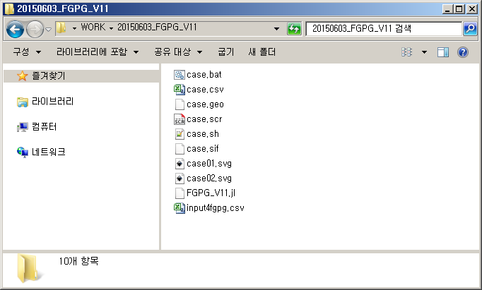
일단 작업하려고 하는 디렉토리를 만들고, 소스코드 및 입력파일을 위와 같이 넣는다.
Juliabox.org 에서 작업할 경우도 역시 마찬가지다.  작업하려는 디렉토리를 만들고 똑같이 넣어두면 된다.

 FGPG_V11.jl 소스코드를 실행하기 위해서는 크게 3가지 방법이 있다.

그냥 cmd 즉 소위 말하는 도스창에서

julia FGPG_V11.jl 

이렇게 커맨드를 직접 때려주는 방법이 있고, 또 다른 방법은 위 그림과 같이 JUNO IDE를 실행시켜서 여기서 실행해 주는 방법이 있다.
마지막으로는 Juliabox.org의 웹브라우저 상에서의 개발환경에서 실행해 줄 수 있다.  Juliabox.org는 기본적으로 IPython Notebook 기반이기 때문에, IJulia Notebook을 자신의 PC에 설치해서 똑같이 해도 된다.

본 예제에서는 위 그림 처럼 JUNO 상에서 실행한다.

 실행 전에 input4fgpg.csv 파일도 열어서 내용 확인하고 적절히 수정해 준 후에, 다시 재 실행하면서 기어 형상 변화를 확인해 갈 수 있을 것이다.

JUNO 에서 소스를 실행하려면, 아래 그림처럼 메뉴 중에서 "Eval All"을 선택해 주면 된다.

참고로, 본 소스코드는 외부 패키지는  PyPlot만 사용한다.
가급적 외부 의존성을 줄여서 간단하게 만들기 위해서이다.
Julia는 JIT 방식이기 때문에, 최초 실행시에는 로딩 및 내부 컴파일 시간이 좀 걸린다.
하지만 두 번째 실행 부터는 상당히 빠르게 수행된다.

실행이 완료되면, 우선 아래와 같은 2개의 그림이 별도 창으로 뜬다.

이것을 보면서 기어의 형상 및 결과로 나오는 주요 치수들을 확인할 수 있다.
기어 사양이 적절치 않다면, input4fgpg.csv 안의 파라미터 값들을 조절해 주면서 반복 실행해 주면 된다.

아울러, 실행이 완료되면 작업 디렉토리 안에 여러 가지 파일들이 만들어져 있음을 볼 수 있다.

우선 case.csv 파일은, 생성된 기어 형상의 원시(Raw) 데이타이다.
이것을 엑셀에서 읽어서 그래프로 그대로 그려줄 수 있다.
또는 Matlab이나 Octave, Scilab 등에서 읽어서 이용할 수도 있다.


case01.svg 및 case02.svg 파일들은 앞서 나타났던 기어 형상 그림들이 파일로 저장된 것이다.
벡터 그림 파일이기 때문에, Inkscape 또는 Adobe Illustrator 같은 것으로 읽어서 활용할 수 있다.
아래의 그림은 Inkscape에서 읽어본 것이다.

case.scr 파일은 AutoCAD Script 파일이다.
AutoCAD 대신 DraftSight에서도 실행 가능하기 때문에, DraftSight에서 실행한 예를 아래 그림과 같이 볼 수 있다.

DraftSight를 실행해서 빈 화면이 나오며느, 화면 아래쪽에 "도면요소 스냅"이 보통 기본적으로 눌러진 상태로 되어 있다.  이것을 마우스로 한 번 눌러줘서 해제 상태로 바꾼다.

"도면요소 스냅"을 해제하는 이유는, 눌러진 상태에서 case.scr 파일을 실행시키면 제대로 그려지지 않고 이상하게 나오기 때문이다.  AutoCAD 에서도 똑같다.

아무튼, 이렇게 실행하면 약간의 수초~십수초 정도의 시간을 소요한 후에 기어 형상이 그려져 있음을 확인할 수 있다.
기어의 치형은 하나의 Spline으로 그려지도록 해 놨다.
또 Addendum 및 Dedendum 값을 비교해서 Internal & External Gear를 자동 판별해서 그려지도록 해 놨다.

이것을 case.dxf로 저장한다.  버전은 R2000~2002 버전으로 적당히 옛날 버전으로 해 두는 습관이 좋겠다.  왜냐면 구버전일수록 여러 소프트웨어를 가리지 않고 잘 열리기 때문이다.

한가지 팁은, R12 버전의 *.dxf 파일로 저장시키면 Spline이 많은 짧은 직선으로 구성된 Polyline으로 바꿔져서 저장된다.  R12 버전에서는 Spline 사양이 없기 때문이다.
이런 특징을 이용해서, Spline 궤적을 생성할 수 없는 공작기계로 가공할 경우에 (구형 와이어 방전 가공기나 밀링머신들은 Spline 궤적 보간 기능이 없고, 오로지 원호 보간 기능만 지원된다.  최신 기계들은 대부분 Spline 보간 기능이 있다.) 대응 가능할 것이다.

한편, case.bat 및 case.sh 파일은 각각 윈도우 및 리눅스용 해석 스크립트이다.
이 파일들을 실행시키면 PC에 이미 Gmsh 및 Elmer가 설치되어 있고 또 path가 잡혀 있는 경우에 한해서 이상없이 FEM 해석이 실시될 것이다.

Batch 파일의 스크립트 내용은 별것 없다.  위 그림과 같다.
순서대로 명령을 실행하는 것이다.
리눅스용 case.sh 파일 역시 같은 동작을 하도록 리눅스용 Bash 쉘에 맞춰서 내용이 들어있다.

gmsh -2 case.geo 명령은, case.geo 형상 파일을 이용해서 gmsh 프로그램으로 2차원 매쉬를 생성하라는 것이다.
매쉬 생성에는 수십초 이상이 소요될 것이다.  커맨트창이 떠서 진행 상황이 확인될 것이다.

gmsh 작업이 끝나면, case.msh 파일이 생성된다.

참고로, case.msh로 만들어지는 매쉬의 특성은, Delaunay 삼각형 자동 생성 알고리즘으로 2nd Order 조건으로 먼저 생성된 후에, Recombine 옵션을 줘 놨기 때문에 삼각형들을 합쳐서 사각형으로 바꿔준다.  따라서 결과물로 나오는 매쉬는 2nd Ordered Quad Mesh가 된다.

매쉬의 조밀함은 input4fgpg.csv 내용 중에서 Segmentation 값들을 올려주면 더 조밀하게 할 수 있다.  대신 해석시간은 기하급수적으로 증가될 것이다.

아무튼 이어서  곧바로 ElmerGrid 명령이 실행된다.  ElmerGrid는 case.msh 파일을 Elmer 전용의 매쉬 포멧으로 바꿔준다.  Elmer용 매쉬 파일은 단일 파일이 아니고, 속성별로 4개의 파일로 저장된다.

따라서 매쉬 생성 결과는, 위 그림과 같이 나타난다.
이어서 곧바로 ElmerSolver가 작동해서 해석을 시작한다.
각종 해석 조건을 설정한 ElmerSolver용 입력파일인 case.sif 파일은 이미 FGPG_V11.jl이 만들어 뒀다.
재질(Carbon Steel), 경계조건의 위치, 힘의 강도(100N)은 상수로 고정시켜 놨기 때문에 소스를 보고 수정해야 바꿀 수 있다.  일단은 잘 되는지 보기 위해 편의상 상수로 뒀다.

아무튼 이에 따라 ElmerSolver가 수행된다.  커맨드창에 나타나는 숫자들은 수렴 오차이다.  수렴오차를 계속 줄여가다가 설정된 오차값 안에 들어오면 해석이 완료되도록 되어 있다.

한참 기다리면 최종적으로 완료된다.  본 예제에서는 해석시간이 406.28초 걸렸다.

이제 어떤 파일이 생겼나 확인해 보면, case_output.msh 파일이 생겨나 있는 것을 확인할 수 있다.  물론 ElmerSolver 결과 파일인 case.ep 역시 함께 생성되어 있다.
이들 파일이 생성된 후에 자동으로 Post Processor로서 gmsh가 실행되어 결과 파일을 띄워준다.

gmsh는 처음 다뤄보는 사람이면 GUI 체계가 좀 생소해서 막막할 수 있는데, 기능들 자체는 매우 단순하다.  이리저리 보면서 건드려 보면 쉽게 습득 가능할 것이다.
일단 본 화면에서는 기본적으로 결과데이타 8가지가 한꺼번에 겹쳐서 보이므로 번잡스럽다.
6번이 VonMises 응력 데이타이므로, 이것을 제외하고 전부 Uncheck 한다.

일단 메뉴에서 Option을 선택해서 화면 상태를 조정해 줄 수 있도록 옵션을 건드려 본다.

Mesh의 Visability 중에서 Surface Edges, Volume Edges를 Uncheck 하면 좀 깔끔해진다.

그리고, Filled iso-values를 선택해서 등고선식으로 보이도록 해 본다.

등고선 단계는 50단계 정도로 해 본다.

그러면 좀 볼 만 하다.  다만 몇 개의 거슬리는 포인트들이 보인다.

거슬리는 포인트는 위 그림처럼 Points를 Uncheck 하면 안보이게 된다.

결과 확인.  그림은 캡춰하거나 다른이름으로 저장할 때 그림포멧으로 지정하면 된다.

이제 7번 Displacement를 본다.

상태 확인하고...

등고선식으로 보이도록 해 보고...

Displacement Factor를 크게 높여서 변형되는 형상을 과장해서 확인해 본다.
이런 식으로 결과 확인이 가능하다.


한 편, 앞서 만들어둔 기어 형상 2D CAD 파일인  case.dxf 파일을 3D CAD에서 읽어들여 모델링해 본다....

일단 FreeCAD에서 잘 되는지 확인.

FreeCAD를 최초로 띄우면 위 그림처럼 나온다.

빈 파일에 case.dxf를 Import 시킨다.

최초에 FreeCAD에는 dxf Reader가 내장되어 있지는 않으나, 우와 같은 창이 뜨면 Yes 해 주면 자동으로 스크립트를 설치해서 읽어들인다.  dxf Reader 부분의 저작권 조건이 달라서 FreeCAD 설치본에 포함하지 못했다고 한다.  (FreeCAD v0.15 기준)

읽어들이는데 성공하면 위 그림과 같다.
간단하게는 이것을 Extrude 시켜서 모델링 하면 된다.

일단은 외곽 라인 부분을 Extrude 해 주는데 일단 Solid가 생성되도록 체크해 준다.

또 기어 치형 부분도 Solid로 Extrude 해 준다.

마지막으로, 생성된 2개의 Extrude Feature를 Boolean Cut 해 준다.
그러면 이상없이 만들어진 모습을 볼 수 있다.
이 파일을 *.step 포멧으로 저장 가능하다.

한편, 프로페셔널하게 쓰는 상용 3D CAD에서도 잘 되는지 확인해 본다...

잘 된다.  모델링 과정 설명은 생략한다.  대충 해 본 거라서..
재밌게 응용해 보기 위해 각도를 살짝 틀어서 Scew를 줘 봤다.  헬리컬기어 느낌이 난다.

이런식으로 응용하면, 상당히 엄밀한 Bevel Gear 및 Bevel Spiral Gear 모델링도 가능할 것이다.




추후에 본 프로그램의 버전업 계획은 아래와 같다.


1. 언더컷 자동 감지 및 겹치는 라인 자동 제거
2. 이끝단 살 소멸 자동 감지 및 겹치는 라인 자동 제거
3. 치형 수정(End Tip Relief) 기능 추가 (Linear Type)
4. 해석 속도 증가를 위해 기어 전체를 해석하지 않고, 3개 정도의 Teeth만 살려서 해석할 수 있도록 수정
5. Theory 및 User Manual 작성


요즘 시간이 점점 쪼들리고 있는데, 신속하게 가능할지는 잘 모르겠다.

이상 끝!